Top 25 Microsoft Excel Formulas You Should Know

Excel has been used in various task and application for a very long time. Excel is an excellent application and it is highly flexible and compatible. 

MS Excel is widely used by many organizations to record, analyze, and process data.

There are various excel formulas for handling and processing  large data.

It can handle large volume of Data and maintain records.

One of the most basic and widely used features in Excel is the Excel Formula/ Functions.

And everyone using Excel should know these Excel formulas. 

Why is it important to know these MS Excel Formulas?

You may be a talented employee ready to face the challenges at the workplace with the proper education and skill set. But what makes you stand out from the crowd? what makes the employer retain you? Well, it’s not just hard work; you have to be that intelligent employee with the basic skill sets required for day-to-day work. Work smartly with

Almost all companies use Microsoft Excel for various activities like data analysis, data storage,  strategic analysis, generating reports and the list goes on. It is necessary for everyone to learn the basics of Excel. There is a wide range of features used in Excel spreadsheets and one such is Excel formulas. 

What is Excel Formula? 

Excel formulas are used to do mathematical calculations. The users can use the advance excel formulas to do complex calculations. There are two ways to do the calculations in the sheet one is using the ms excel formulas or the functions. 

In common these two words are used interchangeably but technically, it is nothing.

Excel Formula – the equation entered manually by the user.

Example – For the addition of two cells 

= A1+A5

Function – to make it user-friendly excel has pre-made many functions 

For example – In addition, of two cells 

=SUM(A1:A5)

However, both give you the same result it is up to the user whether to use formulas or functions. Excel has over 400 functions, explore them in the Formulas tab in the Excel spreadsheet 

 Every formula entered in the spreadsheet should start with equal =

The Benefits of learning Excel Formulas 

For those who are wondering about learning Excel formulas and spending time on it worth a shot? In a recent survey conducted more than 90% of employees responded that Excel formulas are vital to their job. 

Top 5 Reasons to learn Excel formulas 

• Of course, it makes your job a lot easier 
• Enhancing your skill sets – is always an added advantage 
• Excel Formulas help you better at organizing data in most simple manner

• Making you a valuable employee for the company 
• Increases the efficiency and productivity 

If you have come this way long, hope I have convinced you to learn the Top 25 Excel Formulas. Without further delay, let’s see them 

1. SUM function 

The most widely used function in Excel, allows you to find the total of a particular column or the selected range of cell values. Mathematically it is calculated to find the total added value (addition) 

Formula =SUM(num1,num2,…)

Example

To find the total amount 

Under the Amount column for Fruit (cell B6), enter =SUM(B2:B5), or type =SUM(, then select that range with the mouse, and press Enter. This will sum the values in cells B2, B3, B4, and B5. Your answer should be 170.

AUTOSUM 

Now let’s try AutoSum. Select the yellow cell under the column for the Amount  (cell B6), then go to Formulas > AutoSum > select SUM. You’ll see Excel automatically enter the formula for you. Press Enter to confirm it. The AutoSum feature has all of the most common functions.

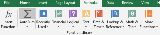
A keyboard shortcut. Select cell B6, then press Alt and =  then, Enter. This automatically enters SUM for you.

2. AVERAGE function

The AVERAGE function is used to get the average of numbers in a range of cells. 

Formula =AVERAGE(num1,num2,..)

Select cell B6, and enter an AVERAGE function by typing =AVERAGE(B2:B5). 

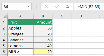
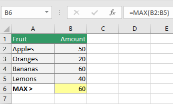
3. MIN and MAX functions

The MIN function is used to get the smallest number in a range of cells.

The MAX function is used to get the largest number in a range of cells.

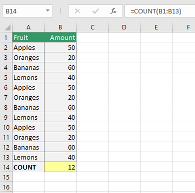
4. COUNT 

The COUNT function allows you to find the total count of entries in the cells that contain numbers. 

Formula =COUNT(value1,value2,..)

Example 

To count the number of cells or array of numbers in B cell, select B14 and enter =COUNT(B1:B13). You can see the count of the cell which has a number alone taken. 

If you need to count the cells, which contain all the values like numbers, text, and any other data format, you can use COUNTA() this does not include the blank cells 

COUNTBLANK() to count the cells that are blank 

5. IF statements 

IF statements let you make logical comparisons between conditions. It generally says that if one condition is true do something, otherwise do something else. The formulas, return text, values, or even more calculations.

Formula =IF(Logical_test,[value_if_true],[value_if_false]

For Example

In cell B2 enter =IF(A2=”Apple”,TRUE,FALSE). The correct answer is TRUE. 

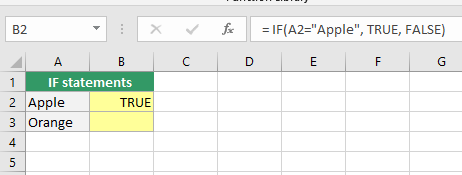
Apply the same formula to B3. The answer here should be FALSE because orange is not an apple.

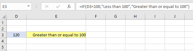
Try another example by looking at the formula in cell E3. We got you started with =IF(D3<100,”Less than 100″,”Greater than or equal to 100″). What happens if you enter a number greater than or equal to 100 in cell D3?

Note: TRUE and FALSE are different from other words in Excel formulas in that they don’t need to be in quotes, and Excel will automatically capitalize them. Numbers need not be in quotes either. Regular text, like Yes or No, should need to be in quotes like this:

=IF(C3=”Apple”,”Yes”,”No”)

6. Conditional Functions – SUMIF 

Conditional functions let you sum, average, count, or get the min or max of a range based on a given condition, or criteria you specify. Such as, out of all the fruits on the list, how many are apples? Or, how many oranges are the Florida type

Formula =SUMIF(range,criteria,[sum_range])

Example 

SUMIF lets you sum in one range based on specific criteria you look for in another range, like how many Oranges you have. Select cell E16 and type =SUMIF(D2:D13,D16,E2:E13). 

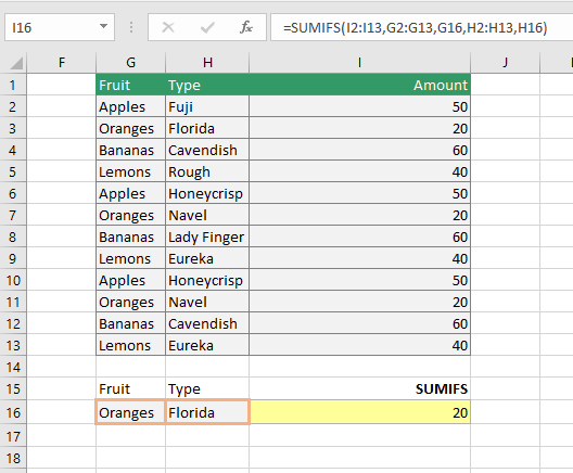
SUMIFS is the same as SUMIF, but it lets you use multiple criteria. 

Formula =SUMIFS(sum_range,criteria_range1,criteria1,criteria_range2…..)

So in this example, you can look for Fruit and Type, instead of just by Fruit. Select cell I16 and type =SUMIFS(I2:I13,G2:G13,I16,H2:H13,H16).

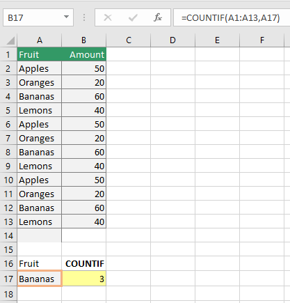
7. COUNTIF 

The function COUNTIF is used when you are required to count cells with specified criteria.

Formula =COUNTIF(range,criteria)

Example 

To count the cell that contains a specific fruit name like Banana, you need to select cell B17 and enter =COUNTIF(A1:A13,A17)

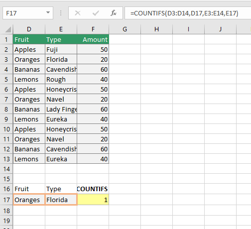
COUNTIFS 

COUNTIFS is the same as SUMIF, but it lets you use multiple criteria. 

Formula =COUNTIFS(criteria_range1,criteria1,..)

So in this example, you can look for Fruit and Type, instead of just by Fruit. Select cell F17 and type =COUNTIFS(D2:D13,D17,E2:E13,E17). 

8. AVERAGEIF 

The AVERAGEIF in Excel returns you the average value in a range with the specified criteria. The specified criteria can be numbers, strings, or references. 

Formula =AVERAGEIF( (range, criteria, [average_range])

Example: The average price of the lemons is returned by entering =AVERAGEIF((A2:A13,A16,C2:C13)

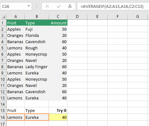
In the second example, we have got the average price of Fruits which is more than the cost of 20 by entering =AVERAGEIF(C2:C13,”>20″)

9. TODAY

TODAY function gives you Today’s date. These are live functions, so whenever you open the workbook, it will have an updated date. Enter =TODAY() in the cell. 

Add Dates – Let’s say you want to know the bill due date, or when you need to return a book. You can add days to a date to find out. In cell B5, enter a random number of days. In cell B6, we added =B2+B5 to calculate the due date today.

10. Ceiling and Floor function 

The Excel CEILING function rounds up to the nearest given multiple numbers. Use CEILING(number) always to ROUND UP the value 

Example 

In the below sheet, we have used CEILING to round up the rate (number) to the multiple of 5 (significance). In cell B2 enter =CEILING(A2,5)

FLOOR 

Excel FLOOR function is the same but rounds down to the nearest given multiples. The FLOOR() is always used to ROUND DOWN the value 

Example 

In the below sheet we have used FLOOR to round down the rate (number) to the nearest multiple of 5 (significance). In cell B2 enter =FLOOR(A2,5)

11. VLOOKUP 

VLOOKUP is the most famous and widely used function, it is the Vertical Lookup in Excel. As the name suggests it is the Excel function that helps to look up specified values vertically. It helps you look up for value in the left column and then returns information in another column to the right if it finds a match. 

Formula =VLOOKUP(lookup_value,tabe_array,col_index_num,[range_lookup]

Example 

In cell B7, enter =VLOOKUP(A7,A2:B5,2,FALSE). The correct answer for Apples is 50. VLOOKUP looked for Apples, found them, then went over one column to the right, and returned the amount.

VLOOKUP Formula structured as 

• A7 – What do you want to look for?
• A2:B5 – Where do you want to look for it?
• 2 – If you find it, how many columns to the right do you want to get a value?
• FALSE – Do you want an exact, or 
• TRUE –  in case of an approximate match?

If VLOOKUP returns an error (#N/A) then it means that the searched value does not exist in the sheet. 

12. CONCATENATE

The word CONCATENATE means to combine. This Excel function simply means to combine different texts from different cells into one cell. The user can do this in two ways either using the build Excel function or the formula 

Formula =CONCATENATE(TEXT1,TEXT2,..)

Example 

=A1&B1 gives the same results as 

=CONCATENATE(A1,B1)

13. LEFT, MID, RIGHT

LEFT function –  To extract the given number of characters from the left of the text 

• Formula – =LEFT(text,num_charc)

MID function – To extract from the middle of the characters in the text, with the given starting position and the number of characters 

• Formula =MID(text,start_num,num_charc)

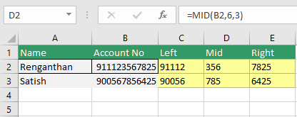
RIGHT function – To extract the given number of characters from the right of the text 

• Formula =RIGHT(text,num_charc)

14. Time functions – NOW 

Excel can give you the current time, based on your computer’s regional settings. You can also add and subtract times. For instance, you might need to keep track of how many hours an employee worked each week and calculate their pay and overtime.

enter =NOW(), which will give the current time, and will update each time Excel calculates. If you need to change the Time format, you can go to Ctrl+1 > Number > Time > Select the format you want.

15. TRIM 

When you receive a worksheet with irregular spaces and the user wants to organize it, then excel has a great function TRIM that cuts out the unwanted spaces in the cell. 

Enter =TRIM(text) to remove the unwanted spaces in the cell

16. UPPER, LOWER, PROPER

• UPPER function – To convert the texts to uppercase. =UPPER()

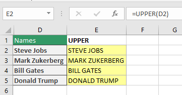
• LOWER function – To convert the texts to lowercase. =LOWER()

• PROPER function – To convert all the improper texts into the correct format 

17. HLOOKUP 

HLOOKUP does the exact same function as VLOOKUP but instead searches for a certain value in the rows in the Excel sheet, whereas VLOOKUP searches the column.

Example: Enter =HLOOKUP(lookup_value, table_array, row_index_num, [range_lookup])

• Lookup value – Apples 
• Table array – the table in which the data is looked up 
• Row index num – the row number in the table array from which the matching value is returned 
• Range lookup – Exact match or approximate match 

18. INDEX and MATCH

INDEX and MATCH are the most popular tools in Excel for carrying out more advanced lookups. This is because INDEX and MATCH are extremely flexible – you can do horizontal and vertical lookups, 2-way lookups, left lookups, case-sensitive lookups, and even lookups based on multiple criteria. If you want to enhance your Excel skills, INDEX and MATCH are musts.

The Excel INDEX function returns the value of a given location in a range or array. You can use INDEX to retrieve individual values, or entire rows and columns. However, the MATCH function is often used together with INDEX to provide row and column numbers.

Formula  =INDEX (array, row_num, [col_num])

For example – in the below list to retrieve data from the required row and column enter =INDEX(A25:C36,3,3)

MATCH 

This Excel function retrieves the location of the specified value from the row, column, and table in the spreadsheet. 

Formula – =MATCH (lookup_value, lookup_array, [match_type])

In the below example we are looking for the position of Kiwi, so enter =MATCH(“Kiwi”,A44:A51,0)

Note: Match type 

• 1 – return the approximate lookup value / Less than the value
• 0 – Exact lookup value 
• -1 –  More than the lookup value 

To sum up, the INDEX returns the value of the given position whereas MATCH returns the position of the lookup value.

The user can combine both INDEX and MATCH functions, 

To look at the value of Grapes in the month of Feb, enter =INDEX(B56:D63,MATCH(“Grapes”,A56:A63,0),2)

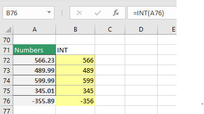
19. INT

In Excel, the INT function is used to remove the decimal from the numbers. This just eliminates the decimals and doesn’t round up or round down to the nearest value. But in case the cell has a negative value then INT acts differently by rounding up/ down 

=INT(Num)

20. TRUNC 

The TRUNC function in Excel is the same as INT but this removes the decimal be it any value entered in the cell.

Formula =TRUNC(number,[num_digits])

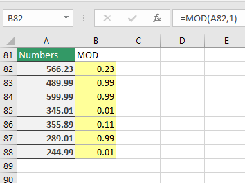
21. MOD 

This Excel function is used in two ways. First, used when you want to extract the decimal part of the value. Second to get the remainder after the division 

Formula =MOD(number,divisior)

22. TRANSPOSE 

This Excel function can be used to transpose your data from Horizontal to vertical or vice versa. 

As it is an array formula user needs to CTRL+SHIFT+ENTER the formula to get the results. 

In the below sheet, the horizontal data has been converted vertically using =TRANSPOSE(array)

• Select the exact space to convert the value 
• Enter the formula 
• Press CTRL+SHIFT+ENTER

23. REPLACE 

This Excel function is used when the user wants to replace a certain specified text or number with a different value or to remove it. The user needs to give the exact location and the new value to get the result 

Formula: =REPLACE(old_text, start_num, num_chars, new_text)

We have two examples- To Remove certain text enter =REPLACE(A98,1,2,””)

To replace a value enter =REPLACE(A103,1,2,91)

24. RAND and RANDBETWEEN

The RAND Excel function retrieves a random number every time an Excel sheet is opened or calculated. 

=RAND() returns a value >= to 0 and < 1

=RAND()*100 returns a number >=0 less than 100

=INT(RAND()*100) returns a random whole number >=0 and less than 100

=RANDBETWEEN(top, bottom) returns a random number within the specified limit 

25. ROW, ROWS, COLUMN, COLUMNS

• ROW – To get the ROW number of any cell
• ROWS – To get the count of the selected array of ROWS
• COLUMN – To get the COLUMN number of the given cell
• COLUMNS – To get the count of the selected array of COLUMNS

In today’s business world, there is a large use of Microsoft Excel. And it is necessary for everyone to learn the basic formula of Excel, which benefits you in so many ways. There is a high demand for Excel skill sets as it is required by vast industries and companies.

If you want to enhance your skills with Advanced Excel knowledge you may check out the course offered.

Henry Harvin 

Henry Harvin offers an Advanced Excel course and it is ranked No. 1 in India. They have trained more than 6000 participants. 

Features of Henry Harvin’s course 

• Get trained by the experts with Multi-Domain exposure. The trainers are certified Excel trainers.
• Complete guidance and support throughout the course
• Gain proficiency in data management and data analysis
• Practical Excel training and application across different industries
• The program includes 11 projects from various domains such as finance, marketing, engineering, etc
• Gain practical Knowledge of Excel Training Tools
• Job assistance to all participants 
• Globally accepted program with Advanced training certification 
• Golden Membership that includes
  • Lifetime Membership of Henry Harvin Accounts Academy for Advanced Excel Certification course.
  • Monthly Bootcamp Sessions  
  • Access to all the recorded sessions 

Learning Benefits 

• Study the tools of Advanced Excel to generate powerful business solutions

• Learn to create a macro in MS Excel

• Learn the importance of the functions in Excel and how it helps to simplify the process

• Gain knowledge on creating Excel templates, tables and charts, financial statement, and many more

• With the Advanced Excel Certification course learn to gather, structure, and present impressive datasets

• Learn to combine the worksheets and workbooks with various features available in Excel

Course Details 

• Duration – 24 hours of live interactive sessions 
• Fees – INR 7500 with EMI INR 833/ month

Conclusion

Excel has been there and will always be there for various purposes and the application has various features and functions that help you to simplify the work. No matter what field you are in, learning the basics of MS Excel will help you in many ways. Those who are keen to know more about the feature and looking to enhance their skills can enroll in the courses offered. 

So what are you waiting for? Keep these Excel formulas handy and improve your productivity. 

FAQ’s

Q1. What are employers looking for in Excel skills?

Ans. The employers seek the basic skills to excel like the commonly used formulas SUMIF, COUNTIF, AVERAGE, VLOOKUP, and keyboard shortcut keys.

Q2. Is there a demand for an Excel expert?

Ans. There is a huge demand for those with Advanced MS Excel skills as the application is widely used across various industries.

Q3. How do I get Excel certified?

Ans. You can take the MOS Excel examination. The minimum passing score is 700 to be certified.

Q4. What is a high-demand Excel skill?

Ans. The most demanded Excel skills are VLOOKUP, INDEX, MATCH, MACROS and VBA, and PIVOT table.

Q.5. Is Excel a good tool for learning financial modeling?

Ans. Yes. Excel is used to create financial models that help with business forecasting and trends. If you’re interested in learning financial modeling, your Excel skills will come in handy.